Batching LLM Requests: Static, Dynamic and Continuous

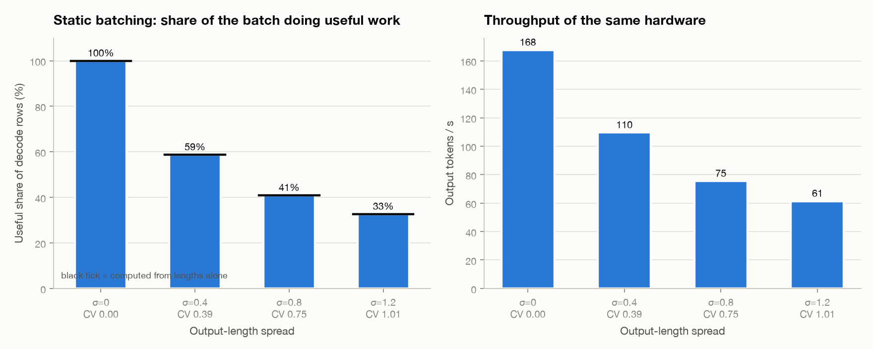
Static batching, when output lengths vary a lot (a coefficient of variation, CV, of about 1: the standard deviation is as large as the mean), keeps only 33% of its decode slots doing useful work. Throughput falls from 168 tok/s to 61 tok/s on the same hardware (measured).

Nothing about the chip changed. The batch just kept computing rows for requests that had already finished. This post is about the three ways of fixing that, and what each one broke.

Part 2 showed that batching decode is almost free, then assumed a tidy batch: everyone starts together and finishes together. It ended with three open items: users who arrive and leave at different times, the cache that grows with torch.cat, and long prefills that stall everyone’s decode. All three are here.

Everything runs on one engine and one serving loop, GPT-2 small on an Apple M1 CPU in fp32. A batching policy is about 30 lines on top of that loop, so any difference between two results is the schedule and nothing else. I label each number measured (real engine, wall clock) or computed (arithmetic from the workload or config). Part 2 covers the roofline, the ridge point, KV sizing and goodput, so I don’t repeat them.

1. Static Batching and Its Zombie Rows

Static batching is the version everyone writes first. Take B requests, run them together, and when the longest one finishes, take the next B.

Time runs left to right. # is a useful row, . is a row computed for a request that has already finished:

slot 0  ##########
slot 1  ####......
slot 2  ######....
        |-- batch 1 --|   batch 2 starts only when slot 0 ends

I gave it every advantage. Saturated arrivals, no prompt padding, a preallocated cache. Only the schedule’s waste is left. The test: 8 slots, 48 requests, output length drawn from a lognormal whose spread (sigma) I swept.

A request that finishes early keeps its row until the longest request in the batch ends. I call these zombie rows. They are computed every step and thrown away.

Slot efficiency is useful rows divided by computed rows. For a static batch it should equal the mean output length divided by the mean of the per-batch maximum. I computed that from the workload before running anything.

Output-length sigma	Length CV (computed)	Slot efficiency, expected (computed)	Slot efficiency (measured)	Avg live rows per step (measured)	Throughput, tok/s (measured)
0	0.00	1.00	1.00	8.0	167.7
0.4	0.39	0.59	0.59	4.7	109.6
0.8	0.75	0.41	0.41	3.3	75.5
1.2	1.01	0.33	0.33	2.6	61.4

The measured efficiency matches the computed one to three decimals. So the loss is purely the schedule, not some engine effect.

Real static batching is worse than this. It would also pad prompts to a common length, which section 5 touches on.

Static batching spends its decode slots on requests that are already done, and the waste grows with the spread of output lengths.

The first idea is that the problem is waiting. If a batch can’t fill, a timeout would let it start anyway.

2. Dynamic Batching: Fixing When, Not What

Dynamic batching adds a timeout. Launch when the queue reaches B, or when the oldest request has waited max_wait seconds. Triton and TorchServe call this dynamic batching.

It bounds the wait to form a batch. It changes nothing after launch. The batch still runs until its longest member ends, so zombie rows stay.

static    wait until 3 requests are queued ------------> launch
dynamic   wait until 3 are queued or max_wait passes --> launch with what is there

slot 0  ##########
slot 1  ####......     zombie rows exactly as before
slot 2  (empty)        smaller batch, shorter wait

I predicted two things. At light load, TTFT drops a lot and batches get tiny. At saturation the timeout never fires, so dynamic equals static. Same workload, two loads, measured:

Load (x decode capacity)	Policy	TTFT p50, s	TTFT p99, s	Throughput, tok/s	Slot efficiency	Avg live rows per step
0.25	static	1.56	5.82	33.9	0.49	3.9
0.25	dynamic, wait 0.1 s	0.68	2.09	35.1	0.65	1.6
0.25	dynamic, wait 0.3 s	0.40	1.76	35.8	0.63	1.7
0.25	dynamic, wait 1.2 s	1.05	2.07	34.7	0.62	2.1
1.5	static	2.92	4.41	84.6	0.49	3.9
1.5	dynamic, wait 0.1 s	3.12	5.11	80.4	0.48	3.2
1.5	dynamic, wait 0.3 s	3.33	6.58	70.4	0.44	3.1
1.5	dynamic, wait 1.2 s	2.78	4.12	87.8	0.49	3.9

The light-load prediction held. A 0.3 s timeout cuts TTFT p50 from 1.56 s to 0.40 s. The price is batches of about 1.7 live rows instead of 3.9, so the batch is barely a batch. Slot efficiency looks better there only because there is little to waste. The best timeout is not the longest: 0.3 s beats both 0.1 s and 1.2 s.

The saturation prediction missed. I expected dynamic to match static. With short timeouts it lost throughput: 70.4 tok/s at 0.3 s against 84.6 tok/s for static, a 17% gap. With 0.6 s and 1.2 s it tied static, slightly ahead.

I don’t have a confirmed reason. My guess is that the short timeout launches a few early batches before the queue has filled, and with only 40 requests in the run that startup cost is a large share of the total. I haven’t logged batch sizes to check.

At the full-size headline workload (section 4), dynamic is no better than static either: 64.9 against 65.2 tok/s, and TTFT p50 of 6.00 s against 5.15 s.

One side experiment shows how much of the later win is just knowing lengths. I added an oracle that groups requests with similar output lengths into the same batch. It cheats, because it reads the true output length, which a real system would have to predict. On the headline workload it lifts throughput from 65.2 to 77.1 tok/s and slot efficiency from 0.39 to 0.59. Continuous batching, next, reaches 107.7 tok/s. Length awareness gets roughly a quarter of the way there (computed from those three numbers). No grouping can give the rest, because a request still waits for its batch-mates.

A timeout fixes how long a batch takes to form. It does nothing about zombie rows, and at saturation it can make things slightly worse.

The fix has to be different in kind. Decide the batch again every step, not once per batch. But my engine can’t do that yet.

3. The Cache Has to Change First

Part 2 left this open. The engine from Part 2 grows the KV cache with torch.cat on every decode step. Cat allocates a new tensor and copies the whole old cache into it.

At batch 16 and context 248, that copies 294 MB per step (computed: 2 x layers x batch x (context + 1) x hidden x 4 bytes). The copy grows with batch times context.

It is also the wrong shape for continuous batching. If the cache is one tensor of shape (batch, tokens), every request in it must advance in lockstep. A request can’t leave and another can’t join mid-flight without rebuilding the tensor.

So the cache becomes a set of slots. Each request owns a fixed row, preallocated to a maximum length. A decode step writes one new K and V into its slot in place. A finished request frees its slot and the next one takes it.

Batch 16, measured on the same machine:

Context	Append via cat, ms	Append in place, ms	Cat copies, MB (computed)	Decode step, cat engine, ms	Decode step, slot engine, ms
32	26.5	0.39	39	291	363
64	8.6	0.28	77	62	56
128	8.0	0.11	152	52	54
192	14.5	0.39	228	58	54
248	11.7	0.11	294	63	55

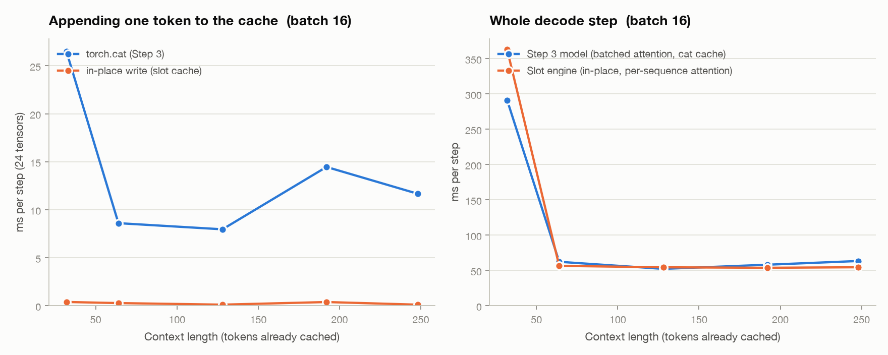
The append itself gets 30 to 100 times faster (ratios computed from the table). The full decode step does not. It is within about 10% either way from context 64 up, and the slot engine is slower at context 32, 363 ms against 291 ms.

The reason is attention. In the slot engine, requests have different lengths, so attention runs as a Python loop over sequences. The cat engine uses one batched attention call. The loop eats most of what the in-place write saves. A real engine fuses it into one variable-length kernel. I haven’t profiled how much the loop costs.

The context-32 row looks like noise to me. Both engines sit near 290 to 360 ms there against about 55 ms everywhere else, and Part 2 measured 39.7 ms for the same batch and context. I haven’t re-run it to find out.

So this is an enabler, not a speedup. It closes the cache-allocation item Part 2 left open, and it makes joining and leaving free. The price shows up in section 7: every slot reserves its full maximum length up front.

The slot cache doesn’t make a decode step faster. It makes the batch something that can change between steps.

4. Continuous Batching

Now the batch can be re-decided every step. That is iteration-level scheduling (the idea from the Orca paper). Before each forward pass, finished requests leave and waiting requests take their slots. Nobody waits for batch-mates, so there are no zombie rows, and TTFT stops including someone else’s decode.

Letters are different requests. Each slot is refilled the step after its request ends:

slot 0  AAAAAAAAAADDDD
slot 1  BBBBEEEEEEEEEE
slot 2  CCCCCCFFFFFFFF
            ^ B ends, E takes its slot on the next step

Because requests in one step are at different stages, the weight matmuls are batched across all of them, and attention runs per sequence. That is why section 3 had to come first.

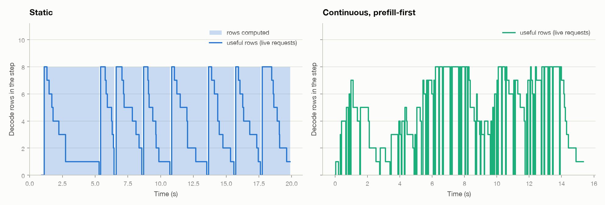
The figure comes from the step 4 run, a workload without long prompts. Static used 49% of its computed rows, continuous used 100%, and throughput went from 85.0 to 110.3 tok/s (measured).

The harder comparison is the headline run: 64 requests, 10% long prompts, 8 slots, offered load 0.8x. All policies see identical arrivals. Goodput, from Part 2, counts tokens from requests that met both limits: TPOT up to 121 ms and TTFT up to 1.01 s. Both limits are relative to this machine’s full-batch decode step.

Continuous batching against static, measured:

• Throughput: 107.7 tok/s against 65.2.
• Goodput: 107.7 tok/s against 11.3. Static misses the TTFT limit for most requests.
• TTFT p50: 0.08 s against 5.15 s. TTFT p99: 0.47 s against 9.75 s.
• Slot efficiency: 1.00 against 0.39.

Static can’t keep up with 0.8x of the nominal capacity. Zombie rows make its real capacity lower, so its queue grows and its TTFT is seconds. Continuous keeps up with the arrivals.

It has a cost, and I predicted it. Inter-token latency (ITL) is the gap between two consecutive tokens of one request. Its p99 is 170 ms for continuous and 45 ms for static. TPOT p50 also rises, from 42 to 51 ms.

The cause is the default policy, prefill-first. When a new request is admitted, that step runs only its prompt. Every request that is decoding produces nothing until it finishes. Static never does this, since it prefills all rows together at the start.

A throughput bar alone would hide this. Averages stay fine, and only the tail gets worse.

Continuous batching removes the zombies and the queueing, and pays for it with stalls in every request’s token stream.

5. Prefill Stalls Decode

A prefill step is compute-bound, and its time grows with the prompt length. While it runs, every decoding request waits.

Two variants, and then the one that works:

• Mixed. Put the new prompts into the same step as the decodes. The decodes don’t skip a step, but the step is as slow as the biggest prompt in it.
• Chunked prefill. Give each step a token budget. Fill it with one token for every running decode first, then a chunk of prompt tokens in whatever budget is left. A prompt that doesn’t fit continues in the next step, with its K and V so far still in its slot.

d is one decode token, P and p are prompt tokens, one step per column group:

prefill-first   d d  PPPPPPPPPPPP  d d     decoders wait through one long step
chunked         d d  d+p d+p d+p d+p       every step is short, the prompt arrives in slices

A step’s time is now bounded by the budget, so ITL has a ceiling no matter how long a prompt is. No engine change was needed. The engine takes a list of (slot, start, tokens), and a decode, a whole prompt and a chunk are the same call with different token counts.

The budget is a trade-off. A long prompt needs about ceil(prompt / budget) steps, so its TTFT rises as the budget shrinks. A very small budget also re-streams all the weights for few tokens. A budget just above the knee of the step-time curve lets decodes ride along for almost nothing.

On the knee: the cost model I fit to measured step times puts it at 38 tokens. Part 2’s reasoning from the ridge in HARDWARE.md (19.8 FLOP/byte on this CPU in fp32) predicted about 40. They roughly agree. I haven’t explained the small gap.

This test has 15% long prompts of 480 tokens, same engine, measured:

Policy	Long-prompt TTFT p50, s	Short-prompt TTFT p50, s	ITL p50, ms	ITL p99, ms	ITL max, ms	Max step, ms	Throughput, tok/s
prefill-first	0.20	0.06	41	241	314	209	72.5
mixed	0.19	0.07	41	178	188	188	72.5
chunked, budget 32	0.64	0.14	39	51	58	58	72.7
chunked, budget 128	0.28	0.07	41	74	96	96	72.8
chunked, budget 512	0.19	0.07	40	178	181	181	72.9

I also ran budgets 64 and 256, which sit between these rows. Throughput is flat across all of them. The budget moves latency around, not throughput.

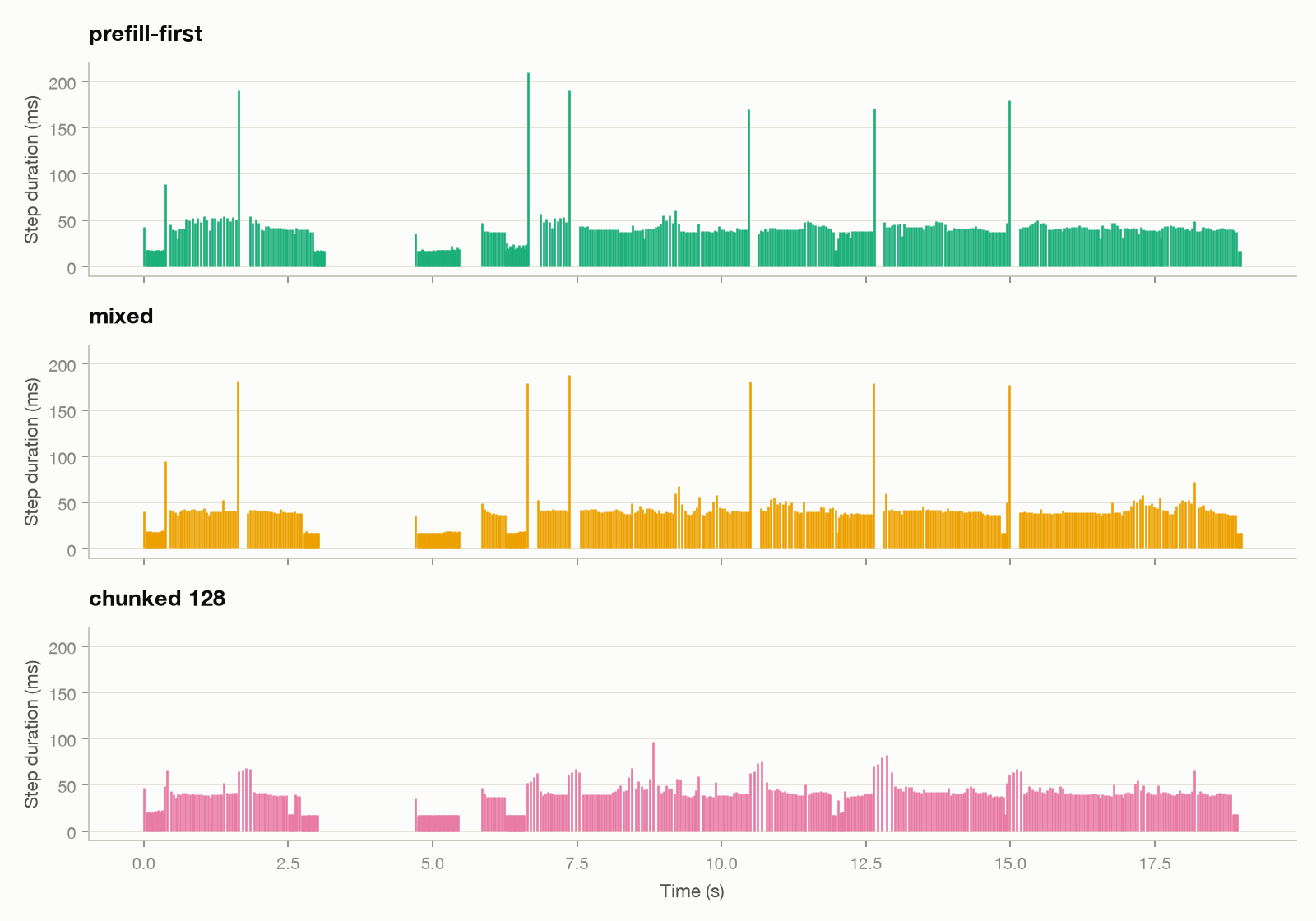
Budget 32 cuts the worst stall from 314 ms to 58 ms, but the long prompts wait 0.64 s instead of 0.20 s. Budget 512 is just mixed.

One aside on prompts. Batching prompts of different lengths into one tensor means padding the short ones. Prefill is compute-bound, so the padding is real work. With a ragged batch, which has no padding, prefill at 62% real tokens ran 1.46x faster than padded (measured). The computed ratio, batch x longest prompt / sum of lengths, was 1.60x. I don’t have an explanation for the gap. Decode barely changed (43 ms padded, 41 ms ragged), because it streams the weights once either way. My padded run feeds the pad tokens through the same kernels, which is a stand-in for a masked tensor, so the real cost of masking could differ.

Chunked prefill caps the stall by spending long-prompt latency, and the budget sets the exchange rate.

6. All Policies Compared

Here are all six policies on the headline workload from section 4, measured on the real engine. The “continuous” row is prefill-first, “mixed” and “chunked” are from section 5 (budget 128), and “bucketed” is the length oracle from section 2.

Policy	Throughput, tok/s	Goodput, tok/s	TTFT p50, s	TTFT p99, s	TPOT p50, ms	ITL p99, ms	Slot efficiency
static	65.2	11.3	5.15	9.75	42	45	0.39
dynamic	64.9	10.5	6.00	11.75	42	47	0.43
bucketed (oracle)	77.1	17.8	2.77	9.98	41	45	0.59
continuous	107.7	107.7	0.08	0.47	51	170	1.00
continuous, mixed	109.7	109.7	0.07	0.27	44	122	1.00
chunked	109.8	109.8	0.08	0.29	44	68	1.00

Chunked is best or tied on throughput and goodput, and well ahead of the other continuous variants on the ITL tail. Its ITL p99 of 68 ms is still above static’s 45 ms. Nothing here removes that gap.

At 0.8x load, the policies that keep up all produce tokens at the arrival rate. Throughput only separates them at saturation, so one load can’t rank them. A sweep over load, output-length spread and slot count can.

Those sweeps are not real-engine runs. Each point would take minutes, and I need about a hundred of them. So I replayed them with a cost model fitted to real step times and checked it against real runs of the same six policies. It ranks policies by throughput well (Spearman 0.94, median error 2%). It ranks TPOT badly (Spearman 0.09). TTFT is in between, with a median error of 16% to 17%. I trust the simulated throughput rankings and distrust its latency details. I did not re-run these sweeps on the real engine, so treat the exact values as approximate.

Load sweep, simulated (median of 3 seeds). Load is a multiple of full-batch decode capacity.

Load	Static, tok/s	Continuous, tok/s	Chunked, tok/s	Static TTFT p99, s	Continuous TTFT p99, s	Chunked TTFT p99, s
0.4	70.4	70.9	70.9	6.63	0.15	0.23
0.8	82.6	140.2	141.3	39.86	2.08	1.24
1.5	84.0	156.9	175.0	61.87	19.43	14.69

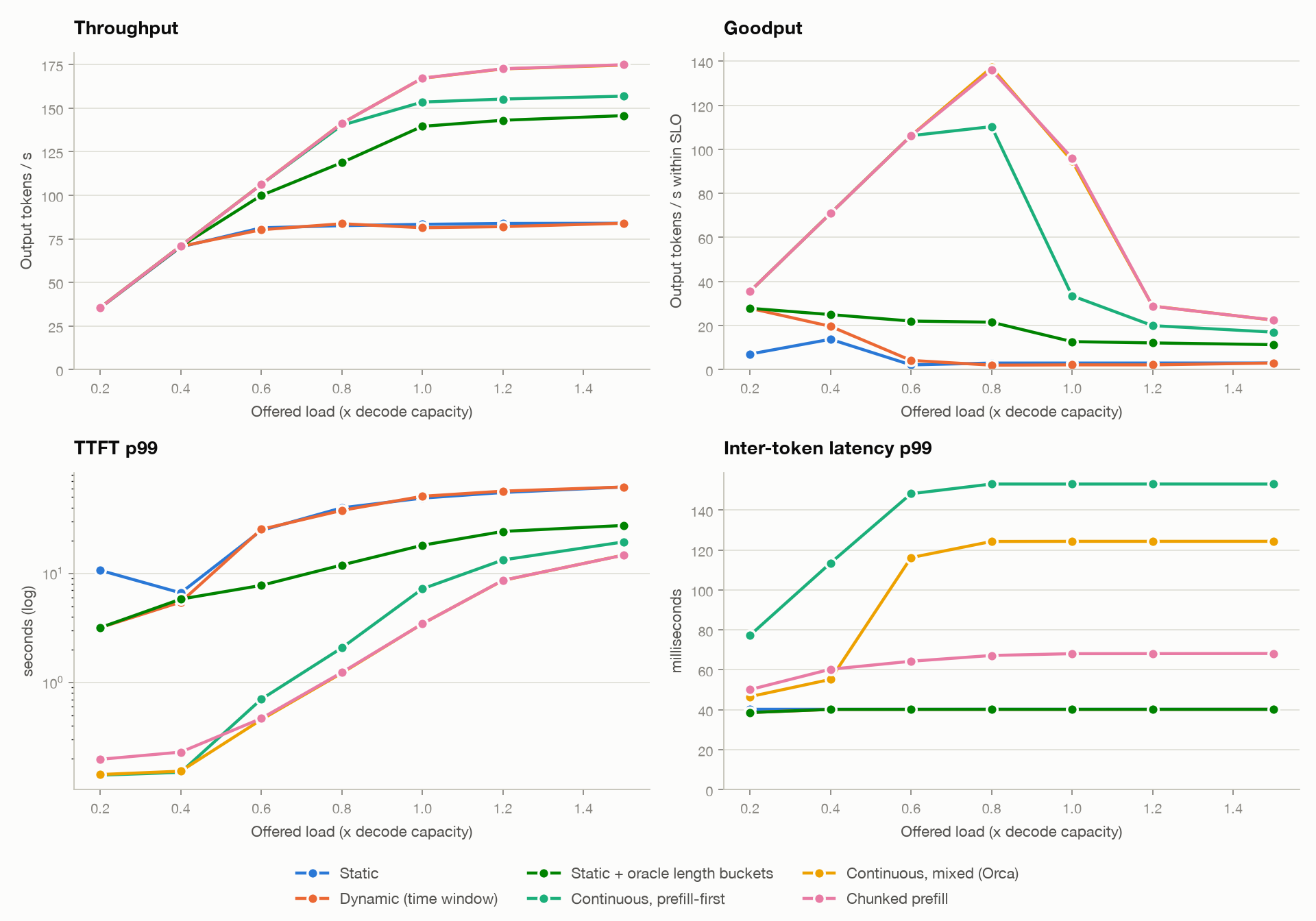
At light load every policy produces the same throughput and the difference is all in latency. Past about 0.6x, static and dynamic flatten near 84 tok/s while the continuous variants keep climbing. Dynamic tracks static at every load. Bucketed sits between them.

The variance sweep, simulated at saturation, shows the same thing as section 1 from the other side. Across output-length CV from 0 to 0.98, static falls from 174 to 70 tok/s, continuous from 167 to 150, and chunked from 179 to 169. Continuous batching mostly shrugs off length spread.

One thing in the plot I haven’t looked into: at the lightest load, static’s simulated TTFT p99 is higher than at 0.4x, which is the wrong direction.

What to pick follows from these results, not from a separate test. Static is fine for an offline job where every output has about the same length, since it has no zombie rows to lose. A timeout (dynamic) only helps when load is light and bursty, and then at the cost of tiny batches. For anything with mixed lengths and live users, continuous batching is the one that holds up, with chunked prefill added when the ITL tail matters.

Continuous batching wins mostly through throughput at saturation and TTFT at every load. Chunked prefill keeps that win without the ITL tail.

7. What Is Still Broken

Throughput keeps rising with concurrency, so more slots look like the answer. Each slot reserves a full-length KV region. Here a slot reserves 416 tokens while the average request uses 122 (computed). 71% of the reserved KV memory is unused.

Slots against reserved memory, simulated at saturation:

Slots	KV reserved, MB (computed)	Static, tok/s	Continuous, tok/s	Chunked, tok/s
2	61	45.0	59.4	60.9
4	123	62.4	101.6	107.8
8	245	84.0	156.9	175.0
16	491	107.9	215.1	244.6
32	981	125.5	267.9	296.9

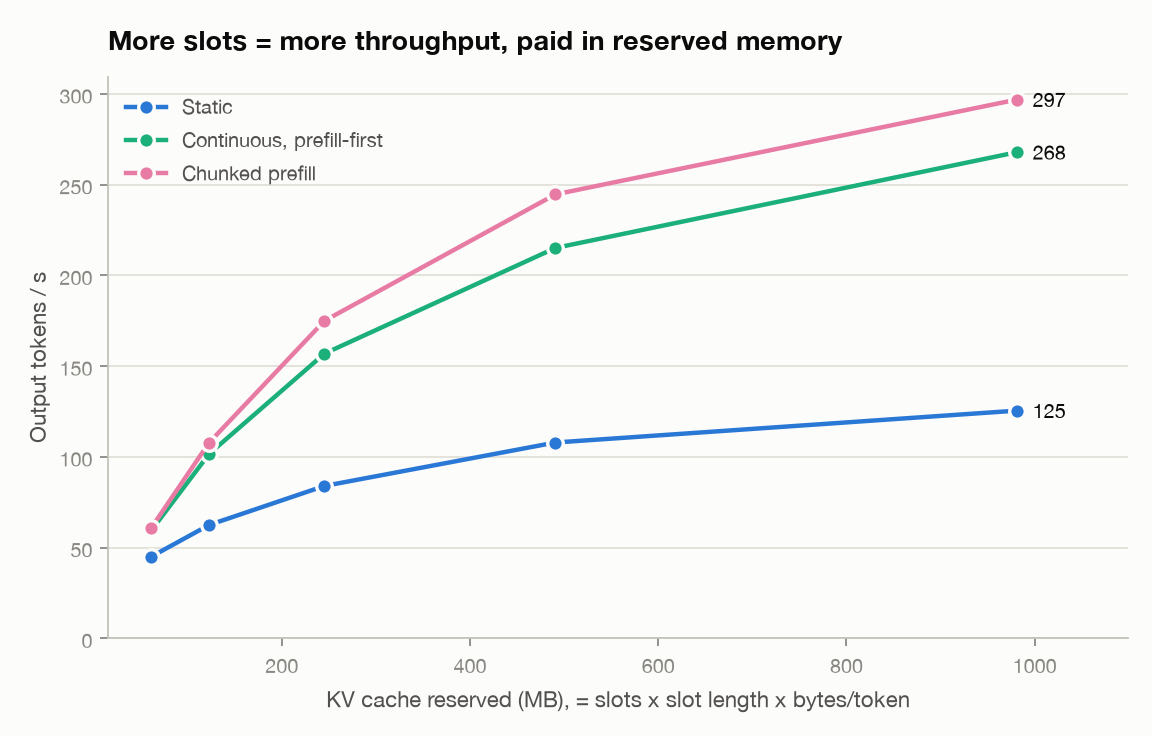
Reserved memory grows linearly with slots, and throughput grows slower. On a GPU the KV cache, not compute, is what caps the batch (Part 2). Reserving the worst case for every request makes that cap arrive much sooner than it should.

Here is what else is still unexplained or unbuilt:

• Attention overhead. Per-sequence attention is a Python loop. I haven’t profiled it against a fused variable-length kernel. That needs a GPU and Triton.
• Small-batch step time. The shape of the step-time curve at small token counts is taken as measured. I haven’t explained it, nor the gap between the 38-token knee and the ridge.
• Dynamic batching at saturation. The 17% throughput miss in section 2 has only a guess behind it.
• Static TTFT in the load sweep. In the simulated sweep, static’s TTFT p99 is higher at the lightest load than at 0.4x. I haven’t looked into it.
• No preemption. When all slots are full, a long request at the head of the queue blocks everyone behind it (first come, first served).
• Lengths come from the workload, not from EOS. Real length distributions are heavier-tailed and correlate with the prompt.
• Greedy decoding only. Per-request sampling parameters and stop strings aren’t batched.
• fp32 only. With fp16 or INT8 the knee moves, since each weight takes fewer bytes.
• No prefix sharing. Requests with a common prompt prefix store it separately.

The next part is about the 71%. A request should get KV memory in small blocks as it grows, not a full-length region up front. That is paged KV memory (PagedAttention), along with block tables, prefix sharing, and what to do with a request when memory runs out.

Code, tests and benchmarks for every step: github.com/sanjay23singh/llm-inference-from-scratch.